OpenOffice works on both Linux and Windows. On Ubuntu, OpenOffice is
the default office suite. On Windows, instead of spending money on
Microsoft Office, download and use Openoffice.
OpenOffice Calc offers pretty much most of the functionalities that are in Microsoft Excel. The following is the list of some Openoffice calc spreadsheet tips and tricks.
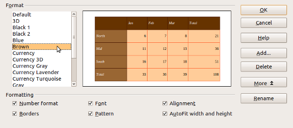
Select the table in the spreadsheet, and click on Menu -> Format -> Autoformat.
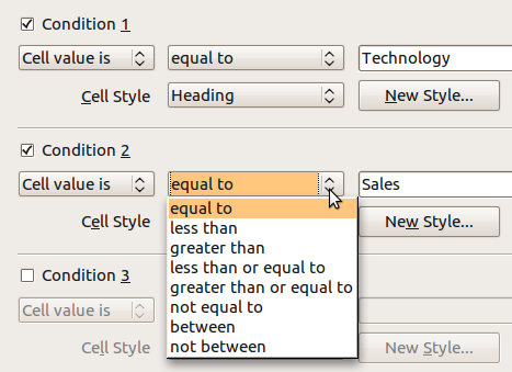
You can also combine multiple conditions using OR/AND conditions. To use this, click on Menu -> Format -> Conditional Formatting.
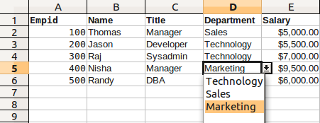
Once you’ve created the list of value, click on any cell in this column, which will show the drop-down list with the values you just created as shown below.
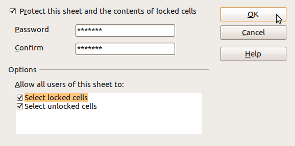
The following shows the protect sheet dialogue. Enter the password to protect the sheet.
Once you protect a sheet, if you try to modify the content of the cells, it will give the message “Protected cells cannot be modified”

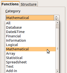
To use the functions, click on the cell where you want the function, and Menu -> Insert -> Functions.
To launch the navigator, Menu -> View -> Navigator.
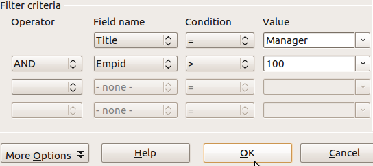
To use standard filter, click on Menu -> Data -> Filter -> Standard Filter, and provide your values as shown below.
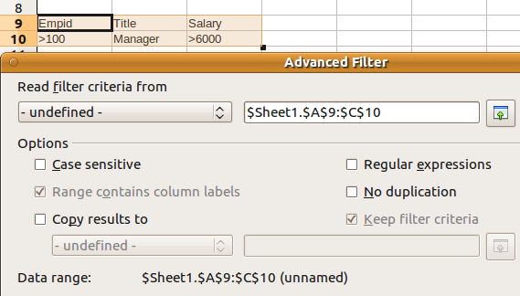
To use advanced filter, click on Menu -> Data -> Filter -> Advanced, and select the range of cells in the spreadsheet that contains the filter information.

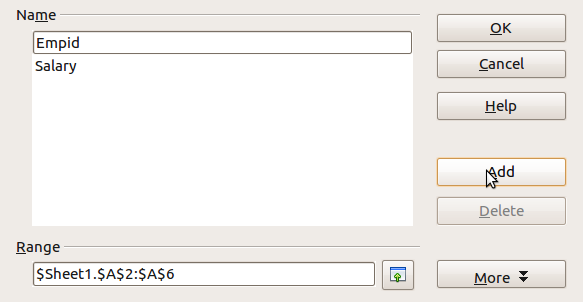
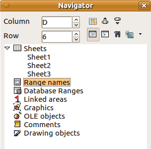
To create a range, select the cells, click on Menu -> Data -> Define Range and give the range name. To select the range, you can use “Navigator”, or Menu -> Data -> Select Range.
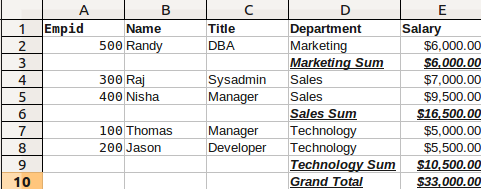
Following is the final output where subtotal of salaries (grouped by department) are automatically displayed.

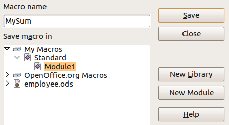
To Record: Click on Menu -> Tools -> Macros -> Record Macros -> [Do all your work] -> Click “Stop Recording” -> Save the macros as shown below.
To Replay: Click on Menu -> Tools -> Macros -> Run Macros -> Pick you macros name -> Run.
OpenOffice Calc offers pretty much most of the functionalities that are in Microsoft Excel. The following is the list of some Openoffice calc spreadsheet tips and tricks.
1. Autoformat Tables
Instead of manually formatting your tables with different font colors and background, you can use one of the builtin table autoformat as shown below.Select the table in the spreadsheet, and click on Menu -> Format -> Autoformat.

2. Conditional Formatting
Using conditional formatting, you can format a specific cell or row only based on a certain condition. For example, if the cell value is “Technology”, you can set a custom background, and font to the cell or row.You can also combine multiple conditions using OR/AND conditions. To use this, click on Menu -> Format -> Conditional Formatting.

3. Create List of Values
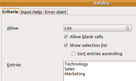
To create list of values based on the data from the columns, select the column, click on Menu -> Data -> Validity. From “Criteria” tab, select “List” in the drop-down for “Allow”. In the Entries text box, enter the list of values that you want to be created as part of the list of values.
Once you’ve created the list of value, click on any cell in this column, which will show the drop-down list with the values you just created as shown below.

4. Protect Sheet or Document
You can protect the current sheet of the whole document, by clicking on Menu -> Tools -> Protect Document -> Sheet (or Document).The following shows the protect sheet dialogue. Enter the password to protect the sheet.

Once you protect a sheet, if you try to modify the content of the cells, it will give the message “Protected cells cannot be modified”
5. Charts
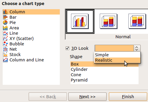
Just like you would expect, you can create various types of charts. Click on Menu -> Insert -> Chart, and get started.
6. Change Status Bar Values
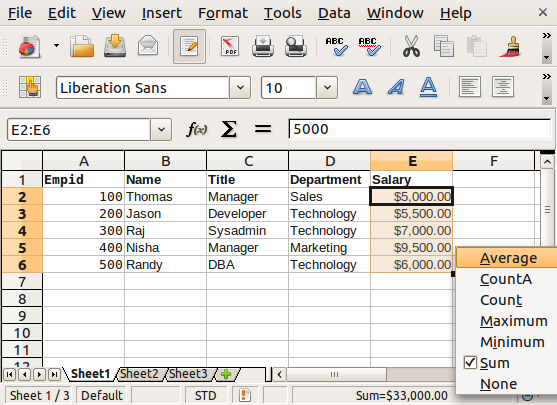
When you select range of cells that contain numeric values, you’ll see the sum of them on the right side of the status bar. You can change this to other values (for example, average) by clicking on the status bar and changing it as shown below.
7. Play Game Inside Calc
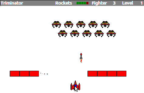
You can play games inside the OpenOffice calc by typing =GAME(“StarWars”) in any of the cell. This will launch the following starwars game. We mentioned this earlier in our Linux Easter Eggs.
8. Meet the OpenOffice Developers
Type =starcalcteam() in any of the cell, which will display the picture of OpenOffice development team members.
9. Use Functions
There are several standard functions available in calc that you can just insert it to a cell and use it. There are almost 100 different functions available that are grouped into more than 10 categories.
To use the functions, click on the cell where you want the function, and Menu -> Insert -> Functions.
10. Navigator
Navigator windows gives a quick way of navigating around the spreadsheet.To launch the navigator, Menu -> View -> Navigator.

11. AutoFilter
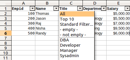
You can automatically create a filter using the 1st row (header row). Click on Menu -> Data -> Filter -> Auto, which will create the auto-filter as shown below. Using this filter, you can filter the rows based on the data in it.
12. Standard Filter
Using standard filter, you can filter data based on 4 conditions. You can combine these conditions using AND / OR conditions.To use standard filter, click on Menu -> Data -> Filter -> Standard Filter, and provide your values as shown below.

13. Advanced Filter
Using advanced filter you can add 8 filter conditions. The advantage of this method is that you can add the conditions in the spreadsheet itself as shown below.To use advanced filter, click on Menu -> Data -> Filter -> Advanced, and select the range of cells in the spreadsheet that contains the filter information.

14. Filter Using Regular Expression
You can also filter data using regular expressions. To do this, click on Menu -> Data -> Filter -> Standard Filter -> More Options -> select the “Regular Expression” check-box.
15. Insert -> Hyperlink
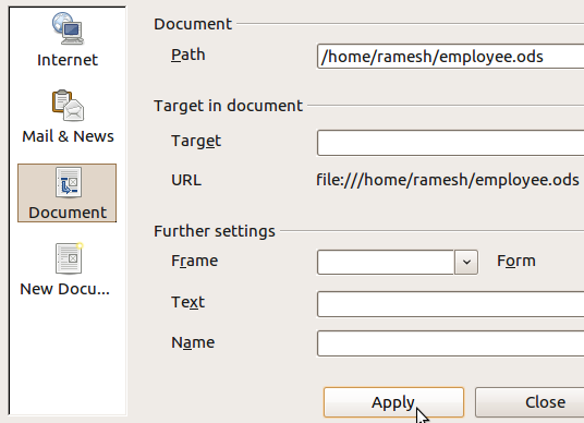
You can insert different types of hyperlinks to a cell. Apart from the standard http:// hyperlink, you can also link to another document as shown below.
16. Format Data
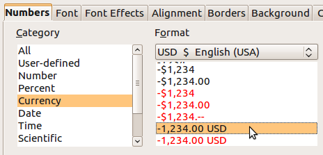
For format cells (or rows, or columns), right mouse click and select “Format Cells”, which will display the following format dialogue.
17. Create and Use Range
You can select a range of cells, and assign a name to them. Later when you use the range name, all those cells will automatically be selected.
To create a range, select the cells, click on Menu -> Data -> Define Range and give the range name. To select the range, you can use “Navigator”, or Menu -> Data -> Select Range.
18. Create Subtotal
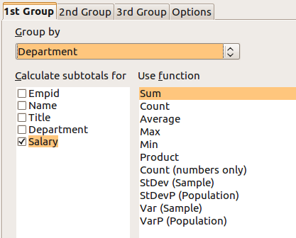
You can automatically create subtotals. Click on Menu -> Data -> Subtotals, which will display following window. From here select the “Group by” column, and the subtotal column. In this example, I want subtotal of salaries of all the employees who belong to a certain department.
Following is the final output where subtotal of salaries (grouped by department) are automatically displayed.

19. Outline
Click on Menu -> Data -> Group and Outline -> AutoOutline, which will display the outline on the left-side of the cells. From here you can click outline indicator to expand or collapse certain group of rows as shown below.
20. Record and Play
Using Macros, you can Record any activities you perform inside the spreadsheet, and replay those activities anytime you want it.To Record: Click on Menu -> Tools -> Macros -> Record Macros -> [Do all your work] -> Click “Stop Recording” -> Save the macros as shown below.
To Replay: Click on Menu -> Tools -> Macros -> Run Macros -> Pick you macros name -> Run.


No comments:
Post a Comment